Aerial manipulators unite the agility of drones with the dexterity of robotic arms. But when the manipulator moves, the drone’s flight dynamics shift instantly — the center of mass changes, and gravity pulls differently on every link. To keep everything stable, a controller must account for these coupled dynamics.
A practical and elegant solution: PD + gravity compensation.
The Problem
When a manipulator is attached to a UAV, its movement alters the total inertia and center of gravity of the system. Traditional UAV controllers assume a rigid body and cannot handle these internal disturbances. A common solution adopted in aerial manipulation is to implement two different controllers, one for the arm and one for the drone, and then expect that the movement of one to be felt as a disturbance by the other. The strategy just mentioned may work when the inertia of the drone is much bigger than the inertia of the arm, but this is not always true. In the context of this project I had to put the boomslang arm on the tilthex drone, so I couldn’t make the simplification explained before.
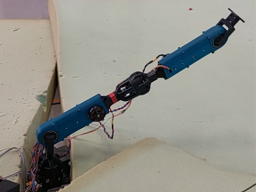
Boomslang
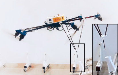
Tilthex
The goal here is to design a whole-body controller that stabilizes both the UAV and manipulator under gravity and makes the movement of the drone compensate for the movement of the arm and vice-versa.
The modeling of the system
The generalized coordinates of the system can be presented as:
\[q = \begin{bmatrix} x \\ y \\ z \\ q_x \\ q_y \\ q_z \\ q_w \\ q_1 \\ q_2 \\ q_3 \end{bmatrix}\]Where:
- \( x \) — Cartesian position along the X-axis (world frame).
- \( y \) — Cartesian position along the Y-axis (world frame).
- \( z \) — Cartesian position along the Z-axis (world frame).
- \( q_x \) — x-component of the orientation quaternion.
- \( q_y \) — y-component of the orientation quaternion.
- \( q_z \) — z-component of the orientation quaternion.
- \( q_w \) — scalar component of the orientation quaternion.
- \( q_1 \) — first joint angle of the arm.
- \( q_2 \) — second joint angle.
- \( q_3 \) — third joint angle.
This way, the generalized coordinate vector \( q \) contains:
- 3D position \( (x, y, z) \)
- Orientation as a quaternion \( (q_x, q_y, q_z, q_w) \)
- Internal joint configuration \( (q_1, q_2, q_3) \)
And the generalized velocities as:
\[\dot{q} = \begin{bmatrix} v_x \\ v_y \\ v_z \\ \omega_x \\ \omega_y \\ \omega_z \\ \dot{q}_1 \\ \dot{q}_2 \\ \dot{q}_3 \end{bmatrix}\]Where:
- \( v_x \) — linear velocity along the X-axis (world frame).
- \( v_y \) — linear velocity along the Y-axis (world frame).
- \( v_z \) — linear velocity along the Z-axis (world frame).
- \( \omega_x \) — angular velocity around the X-axis (roll rate).
- \( \omega_y \) — angular velocity around the Y-axis (pitch rate).
- \( \omega_z \) — angular velocity around the Z-axis (yaw rate).
- \( \dot{q}_1 \), \( \dot{q}_2 \), \( \dot{q}_3 \) — joint angular rates.
The generalized velocity vector \( \dot{q} \) contains:
- Linear velocities \( (v_x, v_y, v_z) \)
- Angular velocities \( (\omega_x, \omega_y, \omega_z) \)
- Joint rates \( (\dot{q}_1, \dot{q}_2, \dot{q}_3) \)
Finally, the generalized acceleration vector is:
\[\ddot{q} = \begin{bmatrix} \dot{v}_x \\ \dot{v}_y \\ \dot{v}_z \\ \dot{\omega}_x \\ \dot{\omega}_y \\ \dot{\omega}_z \\ \ddot{q}_1 \\ \ddot{q}_2 \\ \ddot{q}_3 \end{bmatrix}\]Where:
- \( \dot{v}_x, \dot{v}_y, \dot{v}_z \) — linear accelerations.
- \( \dot{\omega}_x, \dot{\omega}_y, \dot{\omega}_z \) — angular accelerations.
- \( \ddot{q}_1, \ddot{q}_2, \ddot{q}_3 \) — joint accelerations.
With all coordinates defined, their evolution is expressed as:
\[M(q)\,\ddot{q} + C(q,\dot{q})\,\dot{q} + g(q) = \tau\]Where:
- \( M(q) \) — inertia matrix.
- \( C(q,\dot{q}) \) — Coriolis and centrifugal matrix.
- \( g(q) \) — gravity vector.
- \( \tau \) — generalized force/torque vector.
We can further dissect the above equation in the form below:
\[\begin{bmatrix} M_{bb} & M_{bj} \\ M_{jb} & M_{jj} \end{bmatrix} \begin{bmatrix} \dot{v} \\ \ddot{q}_j \end{bmatrix} + \begin{bmatrix} C_{bb} & C_{bj} \\ C_{jb} & C_{jj} \end{bmatrix} \begin{bmatrix} v \\ \dot{q}_j \end{bmatrix} + \begin{bmatrix} g_b \\ g_j \end{bmatrix} = \begin{bmatrix} f \\ \tau_j \end{bmatrix}\]Then we can finally define:
-
Base velocity vector
\(v = [v_x, v_y, v_z, \omega_x, \omega_y, \omega_z]^T\) Base linear and angular velocities. -
Joint position vector
\(q_j = [q_1, q_2, q_3]^T\) Joint angles. -
Joint torque vector
\(\tau_j = [\tau_1, \tau_2, \tau_3]^T\) Joint torques. -
Body wrench vector
\(f = [f_x, f_y, f_z, \tau_x, \tau_y, \tau_z]^T\) Body wrench.
The control strategy
As suggested by the title, the control strategy chosen here was a simple PD plus gravity compensation. It was implemented by choosing the \(\tau\) to be equal to:
\[\tau = \begin{bmatrix} f \\ \tau_j \end{bmatrix} = g(q) + K_p (q_d - q) + K_d (\dot{q}_d - \dot{q})\]The controller combines gravity compensation with proportional–derivative (PD) feedback to regulate both base and joint motion.
-
Generalized Coordinates
\(q = [x, y, z, q_x, q_y, q_z, q_w, q_1, q_2, q_3]^T\) Represents the full configuration of the system, including the base pose (position and orientation) and the joint angles. -
Generalized Velocities
\(\dot{q}\) Denotes the corresponding time derivatives of the generalized coordinates, describing the system’s motion. -
Desired States
\(q_d, \ \dot{q}_d\) Define the target configuration and velocity the controller aims to track. -
Gravity Vector
\(g(q)\) Models the gravitational effects acting on both the base and the joints. -
Proportional Gain Matrix
\(K_p\) A positive-definite matrix that adjusts the stiffness of the position control response. -
Derivative Gain Matrix
\(K_d\) A positive-definite matrix that shapes the damping behavior, smoothing out velocity errors.
Finally, the closed-loop dynamics can be defined as:
\[M(q)\ddot{q} + C(q, \dot{q})\dot{q} = K_p (q_d - q) + K_d (\dot{q}_d - \dot{q})\]With gravity exactly compensated by ( g(q) ), the resulting dynamics describe a PD-stabilized system, ensuring smooth and stable convergence toward the desired motion.
The torques of the joints can be used as control inputs, but the control inputs of the drone need to be obtained using the following body wrench–input mapping:
\[w = A\,u, \quad w = \begin{bmatrix} f_x\\ f_y\\ f_z\\ \tau_x\\ \tau_y\\ \tau_z \end{bmatrix}, \quad u = \begin{bmatrix} u_1\\ u_2\\ \vdots\\ u_m \end{bmatrix}\]Where:
- \( w \in \mathbb{R}^6 \) — wrench (forces and torques).
- \( A \in \mathbb{R}^{6\times m} \) — allocation matrix.
- \( u \in \mathbb{R}^m \) — actuator inputs \( (\omega^2) \).
Explicitly:
\[u = \omega^2 = \begin{bmatrix} \omega_1^2 \\ \omega_2^2 \\ \vdots \\ \omega_m^2 \end{bmatrix}\]Where \( \omega_i \) is the angular velocity of rotor \( i \).
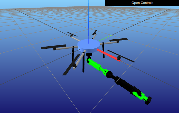
Result
The proposed solution was implemented using the Python package Pinocchio and visualized using Meshcat. Down below, two videos (first with half arm and then with full arm) can be seen of the implemented solution working. The colored arrows represent the different thrusts of each motor.
For now, the system can fly around the workspace and move the arm, but for reliable interaction with the environment an impedance control scheme will be implemented at a later date.
Comments
Comment with your GitHub account.